The Redpoll Platform vs. Standard Machine Learning
Here we demonstrate some of the differences between standard machine learning approaches and the Redpoll discovery platform. This is not meant to be a rigorous analysis, it is meant to showcase the ease of question-asking the Redpoll platform enables. Because we do not wish to spend months on this analysis, when we are forced to make decisions about which model or method to use under the standard machine learning model we will choose what is easiest, not what is best. To put it differently: we will be making nearly every bad, lazy decision to make using standard machine learning seem simpler.
The Dataset
This dataset comes to us from the Union of Concerned Scientists. It is a dataset of Earth satellites and contains information regarding the owner, operator, hardware characteristics, and orbital characteristics of 1167 satellites.
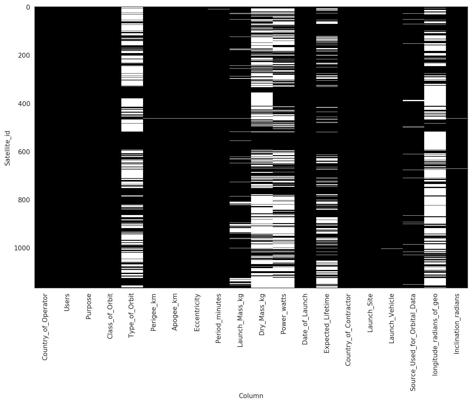
In the figure above the black cells represent present data, and the white cells represent missing data. There are several columns that have more than half their data missing and there are no rows that have zero missing cells. To further complicate matters, the data comprise a combination of continuous-valued columns like Apogee_km (the highest point of an orbit), and categorical-valued columns like Class_of_Orbit, which typically requires manual preprocessing and restrict modeling decisions.
Data Preparation and Training
Redpoll
We give the platform the raw data and ask it to learn, or run. The platform decides what types of data are in each column and builds a model of the dataset. It has no problem with mixed data types or missing data.
>>> import redpoll
>>> redpoll.run(
...     input="data.csv",
...     output="satellites.rp"
... )
Random Forest
The data pose a number of problems for standard machine learning approaches.
First there are continuous columns like period_min (which describes the time in minutes it takes for a satellite to complete and orbit), and there are categorical columns like Country_of_Contractor. Standard machine learning models usually accept one or the other. Deep Learning and Random Forests work only for continuous inputs and outputs, so we'll have to figure out a way to transform the data to fit the model. You might think that we could simply convert the country into an integer and use that. But is Switzerland + 1 = France? No. So what we have to do is to expand the Country_of_Contractor variable into N - 1 binary variables, where N is the number of possible countries. This is called one-hot encoding. Using one-hot for this one column adds 53 variables. Using one-hot for all categorical columns increases our total variable count from 20 to 432. This is really, really bad because for each additional variable, we need exponentially more data to be able to learn. This is the curse of dimensionality.
The second problem is that there are columns with tons of missing data. Random Forests and Deep Learning require complete data. There are a few ways to handle this. We could drop all columns with missing values. This would leave us with zero data. No good. We could fill in the data. Using the mean or median is common for continuous data, but it is biasing because we are feeding the model data we made up; data that were not generated by the process we're trying to learn about. But what about the categorical columns? What is the mean or median country? We could fill in using the most common value (the mode), but this is extremely biasing. We can't just assume that the Class_of_Orbit for every satellites is geosynchronous.
Another option is to create a imputation model that uses the other columns to infer the value of the missing column. So now we are predicting before we predict, and will still have to navigate all the data processing issues to make these imputation models.
Since we must make a decision, we will impute continuous columns with the median and we will impute categorical columns with the mode
>>> import pandas as pd
>>> df = pd.read_csv("data.csv", index_col=0)
>>> df.shape

(1167, 20)

>>> continuous_columns = [
...     'Perigee_km', 'Apogee_km', 'Eccentricity',
...     'Period_minutes', 'Launch_Mass_kg',
...     'Dry_Mass_kg', 'Power_watts',
...     'Date_of_Launch', 'Expected_Lifetime',
...     'longitude_radians_of_geo',
...     'Inclination_radians'
... ]
>>>
>>> target_column = "Expected_Lifetime"
>>>
>>> for col in list(df.columns):
...     # don't mess w/ the target
...     if col == target_column:
...         continue
...
...     if col in continuous_columns:
...         # fill in missing values with mean
...         df[col].fillna(df[col].median(), inplace=True)
...
...     else:
...         # fill in missing values with mode
...         df[col].fillna(df[col].mode()[0], inplace=True)
...
...         # convert strings to categories
...         df[col] = df[col].astype('category').cat.codes
...
...         # create and lable one-hot features
...         one_hot = pd.get_dummies(df[col])
...         one_hot.columns = ["%s_%d" % (col, label) for
...                            label in one_hot]
...
...         # replace categorical column w/ one-hot dummies
...         df.drop([col], axis=1)
...         df = pd.concat([df, one_hot], axis=1)
We split the data into a training set and a test set based on which rows are missing the value of Expected_Lifetime.
>>> df_el_in = df.loc[~df[target_column].isnull(), :]
>>> df_el_out = df.loc[df[target_column].isnull(), :]
>>> df_el_in.shape

(878, 432)
We can see that we have increased the number of features from 20 to 432 — a 21.6x increase in dimensionality.
Now we can break the input/training dataset into inputs (x) and outputs (y), which we can feed to our models for training.
>>> from sklearn.ensemble import RandomForestRegressor
>>>
>>> el_predictor_columns = [col for col in df_el_in.columns if
...                         col != target_column]
>>> el_x = df_el_in.drop(target_column, axis=1)
>>> el_y = df_el_in[target_column]
>>>
>>> rf_el = RandomForestRegressor()
>>> rf_el.fit(el_x, el_y)
Parameter Selection, Feature Selection, and Validation
Redpoll
The Redpoll platform does not require tuning or validating. This does not mean that tuning and validation occur under the hood, out of sight of the user; the mathematical foundations of the Redpoll platform make these procedures unnecessary. That said, it is easy to discover what the platform thinks is important. For example, we visualize which features are important to every possible prediction. This is called structure learning and is one of the most difficult problems in machine learning. The Redpoll platform does this automatically.
>>> rp.heatmap("importance")
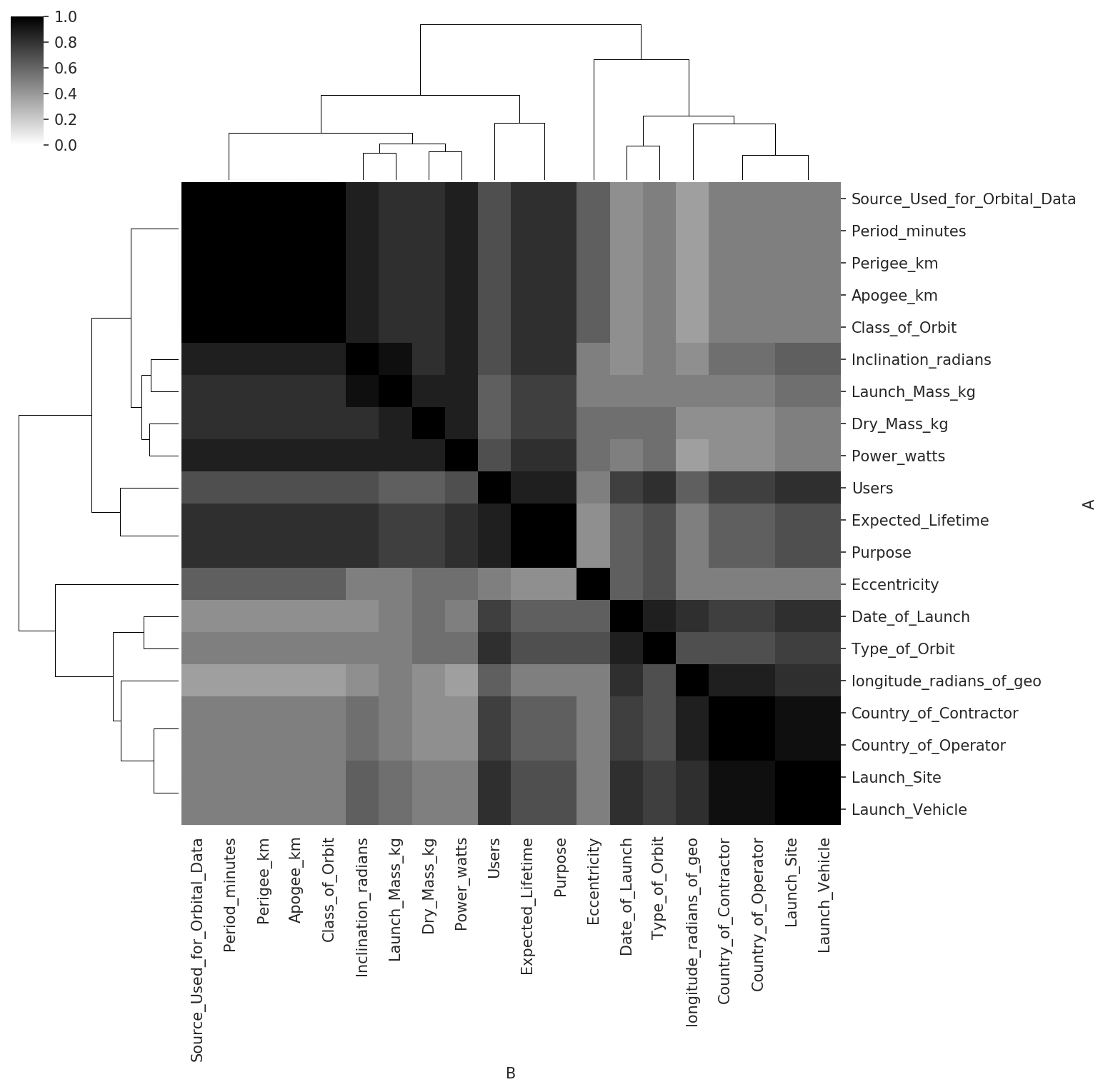
Each cell tells us the probability that a statistical dependence exists between the two columns. A higher number (darker color) indicates higher probability.
Random Forests
The above model was our first pass. It is virtually guaranteed to be suboptimal, especially because we have an average of only two data points per feature. We need to do a couple of things: 1) tweak the random forest parameters, and 2) reduce the number of features so we're not overburdening our data.
If we look at the documentation for the scikit-learn RandomForestRegressor we see that there are 14 parameters to tweak. We're not going to tweak all of those. It's too much work for a questionable payoff. We're going to focus on n_estimators (the number of trees in the forest), criterion (the method for scoring the model), and max_features (the number of features considered). To determine the best parameter set to use we must do a search. We will test a large number of parameter sets and determine which one produces the best performance. We measure performance with cross-validation, which breaks the training set up in to chunks, trains on part of the training set and tests on the left out set. There are many strategies for this, but cross-validation is a must because standard ML models are prone to fit to noise, or to overfit. Overfitting is a common reason that machine learning fails in production.
>>> from sklearn.ensemble import RandomForestRegressor
>>> from sklearn.model_selection import cross_validate
The first thing we need to do is to define the space of parameters for our search. Rather than doing a random search, we're going to pre-define the values for each parameter and perform a grid search. We're going to optimize the sum of test R2 (an arbitrary decision).
>>> import itertools as it
>>>
>>> max_features = ['auto', 'sqrt', 'log2']
>>> criterion = ['mse', 'mae']
>>> n_estimators = [10, 100, 500]
>>>
>>> best_score = None
>>> best_params = None
>>> for params in it.product(max_features, criterion, n_estimators):
...     ftrs, crit, n_est = params
...
...     estimator = RandomForestRegressor(
...         max_features=ftrs,
...         criterion=crit,
...         n_estimators=n_est
...     )
...
...     scores = cross_validate(
...       estimator,
...       el_x,
...       el_y,
...       scoring=('r2',)
...     )
...     score = sum(scores["test_r2"])
...
...     if best_score is None:
...         best_score = score
...         best_params = params
...
...     if score > best_score:
...         best_score = score
...         best_params = params
...
>>> best_params

('sqrt', 'mae', 100)

>>> best_score

2.7996706065580783
This search over 18 parameter sets took about eight minutes to run. We now need to do feature selection. We will pull the feature importances from the random forest and choose the set of 20 features that are most important to the regression. Twenty features being another arbitrary, suboptimal choice made purely to save up work.
>>> el_model = RandomForestRegressor(
...     max_features='sqrt',
...     criterion='mae',
...     n_estimators=100
... )
>>> el_model.fit(el_x, el_y)
>>>
>>> el_importance = pd.DataFrame({
...     "Feature": el_x.columns,
...     "Importance": el_model.feature_importances_
... })
>>>
>>> el_importance = el_importance\
...     .sort_values(by=['Importance'], ascending=False)
>>>
>>> el_features = el_importance.Feature.head(20).values
>>> el_x2 = el_x[el_features]
>>>
>>> scores = cross_validate(
...     el_model,
...     el_x2,
...     el_y,
...     scoring=('r2',)
... )
>>> score = sum(scores["test_r2"])
>>> score

2.6586558550652244
Prediction
Redpoll
We've done our learning already. All we need to do is to spin up an interface to the platform, connect a client, and ask questions. Because we were able to include the data with the missing targets, we can ask to impute those missing targets rather than treat them as predicting hypotheticals. This allows us to exploit the information that exist in those partial data.
>>> server = redpoll.launch(input="satellites.rp")
>>> rp = redpoll.Client("localhost:8000")
>>> el_imputations = rp.impute("Expected_Lifetime")
>>> el_imputations.head()

                      id   uncertainty   Expected_Lifetime
                      --   -----------   -----------------
 Advanced Orion 2 (NR...     0.0581857             8.38443
 Advanced Orion 3 (NR...     0.0497906             8.54544
 Advanced Orion 4 (NR...      0.033794             8.22257
 Advanced Orion 5 (NR...      0.240803             13.8332
 Advanced Orion 6 (NR...     0.0794021             8.10581
Random Forests
This is pretty simple. We have trained and validated our model. Now all we need to do is feed the model the predictor data.
>>> predictors = [col for col in df_el_out.columns if
...               col != target_column]
>>> el_predictors = df_el_out.drop(target_column, axis=1)
>>> el_predictions = el_model.predict(el_predictors)
Classification
Let's try to predict the missing values for a categorical variable, Type_of_Orbit. In standard machine learning predicting a categorical variable is called classification.
Redpoll
Asking another question with the Redpoll platform is as simple as asking the question.
>>> ot_imputations = rp.impute("Type_of_Orbit")
>>> ot_imputations.head()

                       id   uncertainty      Type_of_Orbit
                       --   -----------      -------------
                 AAUSat-3      0.177889    Sun-Synchronous
 ABS-1 (LMI-1, Lockhee...      0.518497    Sun-Synchronous
 ABS-1A (Koreasat 2, M...      0.664371    Sun-Synchronous
 ABS-2i (MBSat, Mobile...      0.575258    Sun-Synchronous
 ABS-7 (Koreasat 3, Mu...      0.523633    Sun-Synchronous
Random Forests
We have to start from square one. We have to go back to the raw data because we filled in the missing values in this column. Then we have to fill in the missing values for the old target, so it can be used as a predictior; and we have to spit the dataset into one set were the target is present (training data), and the set for which the target is missing.
We also need to re-do the parameter search and validation.
First, we'll process the data using the same procedure as above.
>>> df = pd.read_csv("data.csv", index_col=0)
>>> target_column = "Type_of_Orbit"
>>>
>>> for col in list(df.columns):
...     # don't mess w/ the target
...     if col == target_column:
...         continue
...
...     if col in continuous_columns:
...         # fill in missing values with mean
...         df[col].fillna(df[col].median(), inplace=True)
...
...     else:
...         # fill in missing values with mode
...         df[col].fillna(df[col].mode()[0], inplace=True)
...
...         # convert string categories to int codes
...         df[col] = df[col].astype('category').cat.codes
...
...         # create and lable one-hot features
...         one_hot = pd.get_dummies(df[col])
...         one_hot.columns = ["%s_%d" % (col, label) for
...                            label in one_hot]
...
...         # replace categorical column w/ one-hot dummies
...         df.drop([col], axis=1)
...         df = pd.concat([df, one_hot], axis=1)
...
>>> df_co_in = df.loc[~df[target_column].isnull(), :]
>>> df_co_out = df.loc[df[target_column].isnull(), :]
>>>
>>> df_co_in.shape

(521, 425)

>>> df_co_out.shape

(646, 425)
Now we do parameter selection and cross-validation. The parameters and objective change a bit because we're doing classification rather than regression, but the procedure is the same.
>>> co_x = df_co_in[[col for col in df_co_in.columns if
...                  col != target_column]]
>>> co_y = df_co_in[target_column]
>>> from sklearn.ensemble import RandomForestClassifier
>>>
>>> max_features = ['auto', 'sqrt', 'log2']
>>> criterion = ['gini', 'entropy']
>>> n_estimators = [10, 100, 500]
>>>
>>> best_score = None
>>> best_params = None
>>> all_scores = []
>>> for params in it.product(max_features, criterion,
...                          n_estimators):
...     ftrs, crit, n_est = params
...
...     estimator = RandomForestClassifier(
...         max_features=ftrs,
...         criterion=crit,
...         n_estimators=n_est,
...     )
...
...     scores = cross_validate(estimator, co_x, co_y,
...                             scoring=('f1_micro',))
...     score = sum(scores["test_f1_micro"])
...     all_scores.append(score)
...     if best_score is None:
...         best_score = score
...         best_params = params
...
...     if score > best_score:
...         best_score = score
...         best_params = params

UserWarning: The least populated class in y has only 1 members, which is less than n_splits=5.
  % (min_groups, self.n_splits)), UserWarning)
UserWarning: The least populated class in y has only 1 members, which is less than n_splits=5.
  % (min_groups, self.n_splits)), UserWarning)
UserWarning: The least populated class in y has only 1 members, which is less than n_splits=5.
  % (min_groups, self.n_splits)), UserWarning)
UserWarning: The least populated class in y has only 1 members, which is less than n_splits=5.
  % (min_groups, self.n_splits)), UserWarning)
UserWarning: The least populated class in y has only 1 members, which is less than n_splits=5.
  % (min_groups, self.n_splits)), UserWarning)
UserWarning: The least populated class in y has only 1 members, which is less than n_splits=5.
  % (min_groups, self.n_splits)), UserWarning)
UserWarning: The least populated class in y has only 1 members, which is less than n_splits=5.
  % (min_groups, self.n_splits)), UserWarning)
UserWarning: The least populated class in y has only 1 members, which is less than n_splits=5.
  % (min_groups, self.n_splits)), UserWarning)
UserWarning: The least populated class in y has only 1 members, which is less than n_splits=5.
  % (min_groups, self.n_splits)), UserWarning)
UserWarning: The least populated class in y has only 1 members, which is less than n_splits=5.
  % (min_groups, self.n_splits)), UserWarning)
UserWarning: The least populated class in y has only 1 members, which is less than n_splits=5.
  % (min_groups, self.n_splits)), UserWarning)
UserWarning: The least populated class in y has only 1 members, which is less than n_splits=5.
  % (min_groups, self.n_splits)), UserWarning)
UserWarning: The least populated class in y has only 1 members, which is less than n_splits=5.
  % (min_groups, self.n_splits)), UserWarning)
UserWarning: The least populated class in y has only 1 members, which is less than n_splits=5.
  % (min_groups, self.n_splits)), UserWarning)
UserWarning: The least populated class in y has only 1 members, which is less than n_splits=5.
  % (min_groups, self.n_splits)), UserWarning)
UserWarning: The least populated class in y has only 1 members, which is less than n_splits=5.
  % (min_groups, self.n_splits)), UserWarning)
UserWarning: The least populated class in y has only 1 members, which is less than n_splits=5.
  % (min_groups, self.n_splits)), UserWarning)
UserWarning: The least populated class in y has only 1 members, which is less than n_splits=5.
  % (min_groups, self.n_splits)), UserWarning)
We got a lot of warnings. It seems that the random forest algorithm doesn't like when there is only one example of a class. In this case, the Type_of_Orbits Cislunar and Retrograde each appear only once in the training set.
In any case, we have our best parameter set (unless the warnings mean that the model is compromised) so we continue on to feature selection.
>>> (best_score, best_params)

(4.510531135531136, ('auto', 'entropy', 10))

>>> co_model = RandomForestClassifier(
...     max_features='auto',
...     criterion='entropy',
...     n_estimators=10
... )
>>> co_model.fit(co_x, co_y)
>>> co_importance = pd.DataFrame({
...     "Feature": co_x.columns,
...     "Importance": co_model.feature_importances_
... })
>>> co_importance = co_importance\
...     .sort_values(by=['Importance'], ascending=False)
>>> co_features = co_importance.Feature.head(20).values
>>> co_x2 = co_x[co_features]
>>> scores = cross_validate(co_model, co_x2, co_y,
...                         scoring=('f1_micro',))
>>> score = sum(scores["test_f1_micro"])
>>> score

py:667: UserWarning: The least populated class in y has only 1 members, which is less than n_splits=5.
  % (min_groups, self.n_splits)), UserWarning)
4.6069597069597075
And we get the same warning again. But it seems that reducing the number of features has produced a better-scoring model.
Prediction certainty
How certain are we in our predictions?
Redpoll
As a part of computing the imputation, we have already computed the imputation uncertainty. But what do those numbers mean?
>>> el_predictions.head(3)

                      id   uncertainty   Expected_Lifetime
                      --   -----------   -----------------
 Advanced Orion 2 (NR...     0.0581857             8.38443
 Advanced Orion 3 (NR...     0.0497906             8.54544
 Advanced Orion 4 (NR...      0.033794             8.22257
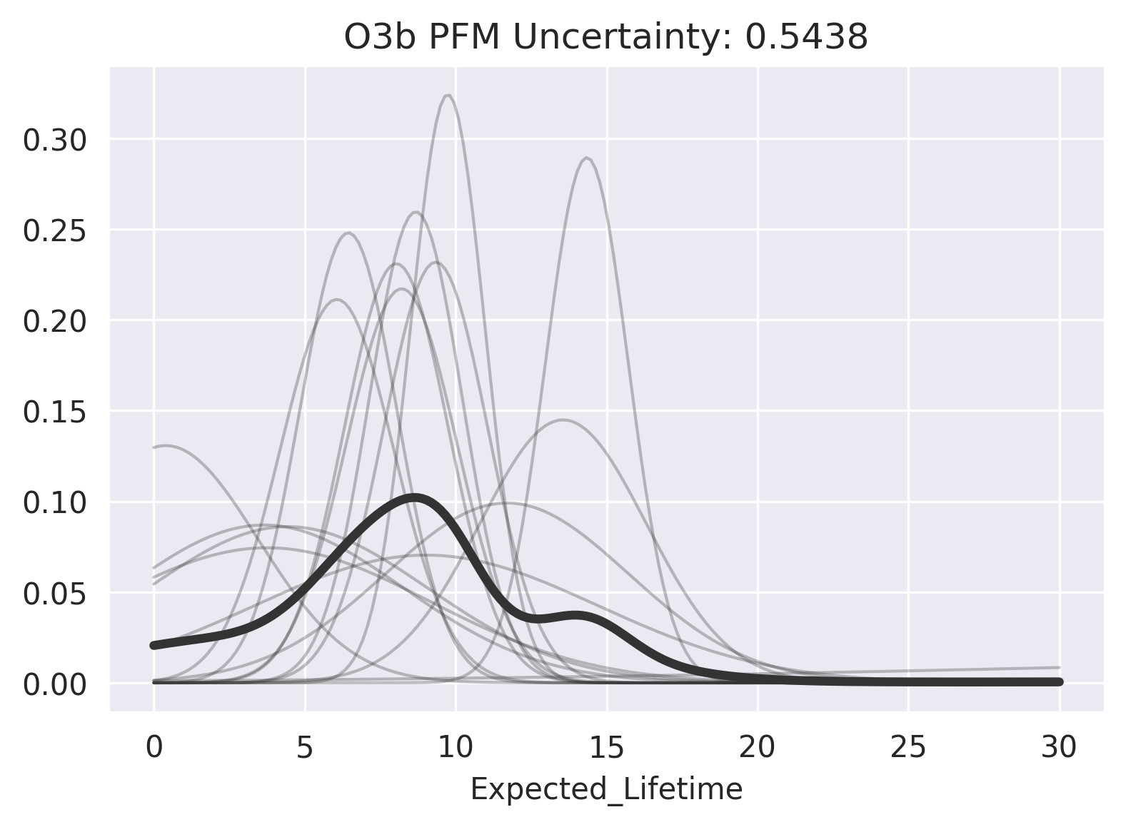
Redpoll's prediction certainty is a measure of the platform's certainty in its ability to model a prediction. It has nothing to do with the variance of the distribution — the model might be very certain there is a high variance. We can visualize impute uncertainty to get a sense of what it means. For a high-uncertainty imputation:
>>> rp.impute_uncertainty(
...     row="O3b PFM",
...     column="Expected_Lifetime",
...     render=True
... );
And for a low-uncertainty imputation:
>>> rp.impute_uncertainty(
...     row="Advanced Orion 4 (NRO L-26, USA 202)",
...     column="Expected_Lifetime",
...     render=True
... );
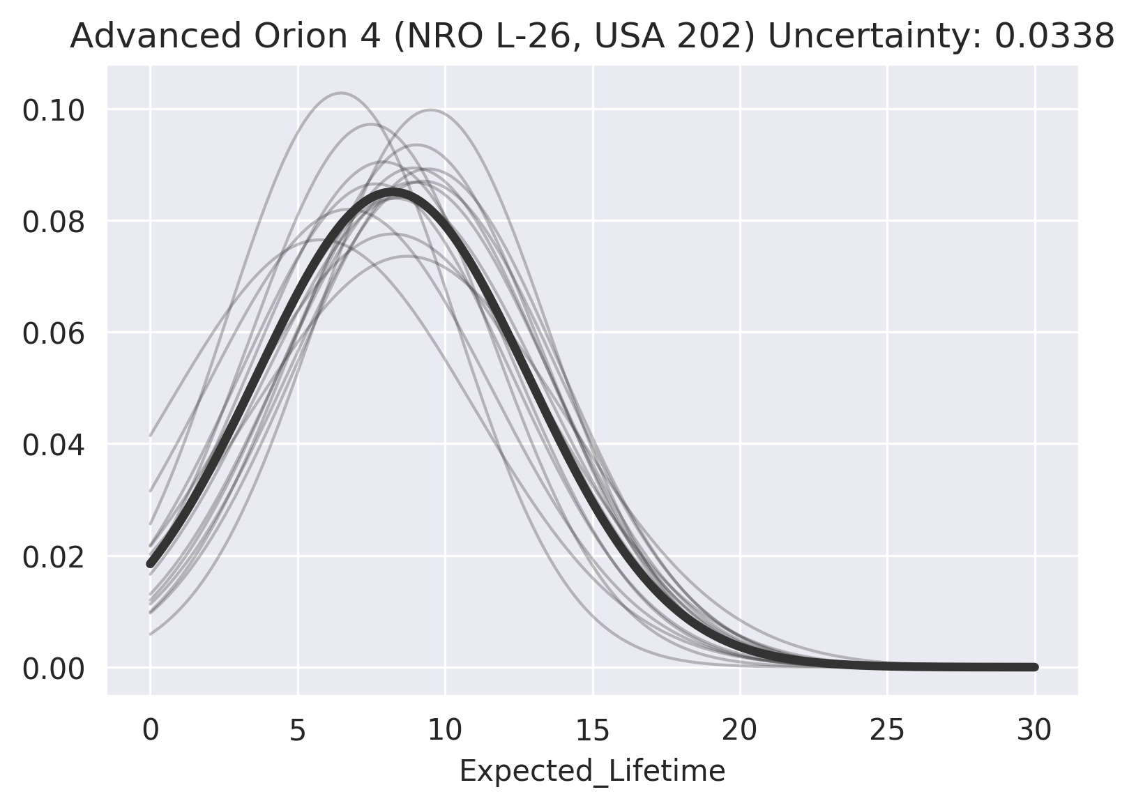
We see that there is a substantial variance in the imputation distribution in both cases, but that the consensus for Advanced Orion 4 (NRO L-26, USA 202) is much higher, thus its imputation has much less uncertainty.
Random Forests
A Random Forest classifier provides a softmax function that produces "probabilities" for each class. These probabilities are not uncertainties — though they are often confused for them. We would like to know the uncertainty of each class over softmax functions.
There are few methods for quantifying uncertainty in random forests, but there is nothing in the machine learning library we're using, so we have to bring in another library, forestci.
>>> import forestci
>>> forestci.random_forest_error(
...     rf_el,
...     el_x,
...     el_predictors,
... )

RuntimeWarning: overflow encountered in exp g_eta_raw = np.exp(np.dot(XX, eta)) * mask
RuntimeWarning: overflow encountered in exp g_eta_raw = np.exp(np.dot(XX, eta)) * mask

array([15.77225733, 16.83583305, 16.14404858, ..., 24.89957166, 16.18654164, 15.23748171])
This gives us a "confidence interval" number for each prediction, but it does not give us a way to visualize what that number means. And there were some warnings. We will hope these warning do not mean our certainty information is compromised.
Anomaly detection
Redpoll
Again, we've done our learning already. We have created a model of satellites, which means we have an idea of how features of satellites affect other features. Because we have this type of intuitive model, it is easy to see when a satellite violates our intuitive model. We say the degree to which a data point violates our expectation is its novelty — or anomalousness.
First, we ask which satellites have unexpected lifetimes.
>>> rp.novelty("Expected_Lifetime")\
...     .sort_values(by=["novelty"], ascending=False)\
...     .head()

                        id   Expected_Lifetime   novelty
--------------------------   -----------------   -------
International Space Sta...                  30   9.62866
                 Landsat 7                  15   5.30769
                  Optus B3                 0.5    4.4782
              Intelsat 701                 0.5    4.2953
                 Sicral 1A                 0.5   4.28725
Redpoll finds that the ISS is an unusual satellite. Low-Earth-Orbit satellites are not meant to last long, and the ISS is has the longest expected lifetime of any satellite in the dataset.
Next, we ask which satellites have an unexpected orbital period.
>>> rp.novelty("Period_minutes")\
...     .sort_values(by=["novelty"], ascending=False)\
...     .head()

                        id   Period_minutes   novelty
--------------------------   --------------   -------
Wind (International Sol...          19700.5   10.9548
      Spektr-R/RadioAstron             0.22   9.18558
Interstellar Boundary E...             0.22   9.16484
Chandra X-Ray Observato...          3808.92   9.14082
Tango (part of Cluster ...             3442   8.89269
The Redpoll platform finds some unusual satellites. Two are reported to orbit the Earth in less than 15 seconds (0.22 minutes). These are data entry errors. Spektr's orbital period is 12769.93 minutes according to Wikipedia. The Wind satellite is another oddity. It sits on a stable gravitational point called a Lagrange point so it doesn't move much, so it has a long orbital period. Using the platform, we have found both outliers and data entry errors.
Random Forests
There is no way to do this with a Random Forest regressor. The standard way that we do this in statistics is to arbitrarily classify all data that are greater than three standard deviations away from the mean as outliers.
>>> pm = df.Period_minutes[~df.Period_minutes.isnull()]
>>> pm_dist = ((pm-pm.mean())/pm.std()).abs()
>>> outliers = pm_dist[pm_dist > 3]
>>> pm = df.Period_minutes.loc[list(outliers.index)]\
...     .sort_values(ascending=False)
>>> pm.head()

                                  id   Period_minutes
                                  --   --------------
 Wind (International Solar-Terres...         19700.45
 Integral (INTErnational Gamma-Ra...          4032.86
     Chandra X-Ray Observatory (CXO)          3808.92
 Tango (part of Cluster quartet, ...          3442.00
 Rumba (part of Cluster quartet, ...          3431.10
Since the data are skewed, this is giving us the satellites with the highest orbital period.
Conclusion
We have seen that the Redpoll Discovery Platform makes discovery trivial. Standard machine learning is built to model questions. This requires an immense amount of effort from the user to find a valuable question and to frame that question in a way that is both compatible with a specific machine learning method, and will not bias the answer. On the other hand, the Redpoll Discovery Platform is built to model data, which means that it is general to data in real-world condition (messy, mixed, and full of holes), which eliminates most data preprocessing; and once the learning is done, the user may any number of questions with very little effort.
Get in touch
Redpoll is deliberate about the organizations with whom we choose to partner. If you’re interested in working with us, please fill out the brief form below and we’ll set up a time to connect!