Machine Learning is often treated as a panacea to any data woes one might have. This is in contrast to the limited capabilities of typical, widely available ML solutions. Almost any model — from the humble perceptron to the formidable, pre-trained VGG-19 deep neural network — is very focused and restricted in its immediate scope. They are trained and tuned to perform one task well. These tend to be of little use for any other goals, even one which is based on the exact same dataset.

In this post, we'll review a simple supervised classification task as it's commonly encountered, and deal with it via traditional ML methods. Then we will extend the scope of what can be performed on such a dataset when Redpoll's Reformer, a holistic AI engine, is applied. The (non-exhaustive) capabilities covered will be:

• Inference (predictions)
• Missing data handling
• Feature importances
• Simulation
• Anomaly detection
• Uncertainty estimation

Gamma Ray Detection with the MAGIC Observatory

In the Canary Islands, off the coast of Western Sahara, there is an observatory consisting of two 17m telescopes whose primary purpose is to detect traces of rare high-energy photons, known as gamma rays. These extra-solar visitors collide with the Earth from fascinating, catastrophic origins. Studying these events (incident angle, energy) can yield insights into the science of faraway cataclysmic events and large astronomical objects.

The problem is that Earth is continuously bombarded by high-energy particles (cosmic rays) that are decidedly not gamma rays, causing a noisy background of gamma ray-like events. Being able to automatically discriminate between real gamma shower events and "hadronic showers" would be very useful, especially since hadronic showers are much more common to occur.

Geometric feature extraction from gamma event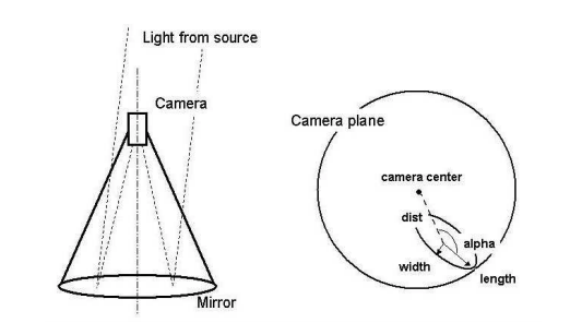

Without going into much detail, these events light up "pixels" of a detector, forming an ellipse. These ellipses can be parametrized by characteristics such as distance from the center of the camera (fDist), length (fLength) and width (fWidth) of the ellipse's axes, and angle of its long axis (fAlpha). There are also metrics representing how bright the pixels are (fSize) and how concentrated that brightness is (fConc). You can find the dataset and the full definition of the features at the UCI Machine Learning Repository

import pandas as pd
import seaborn as sns

df = pd.read_csv("magic04.data", index_col=0)
sns.pairplot(
    data=df,
    vars=["fLength", "fWidth", "fConc", "fAlpha", "fM3Trans"],
    hue="class",
    kind="kde",
    corner=True,
)

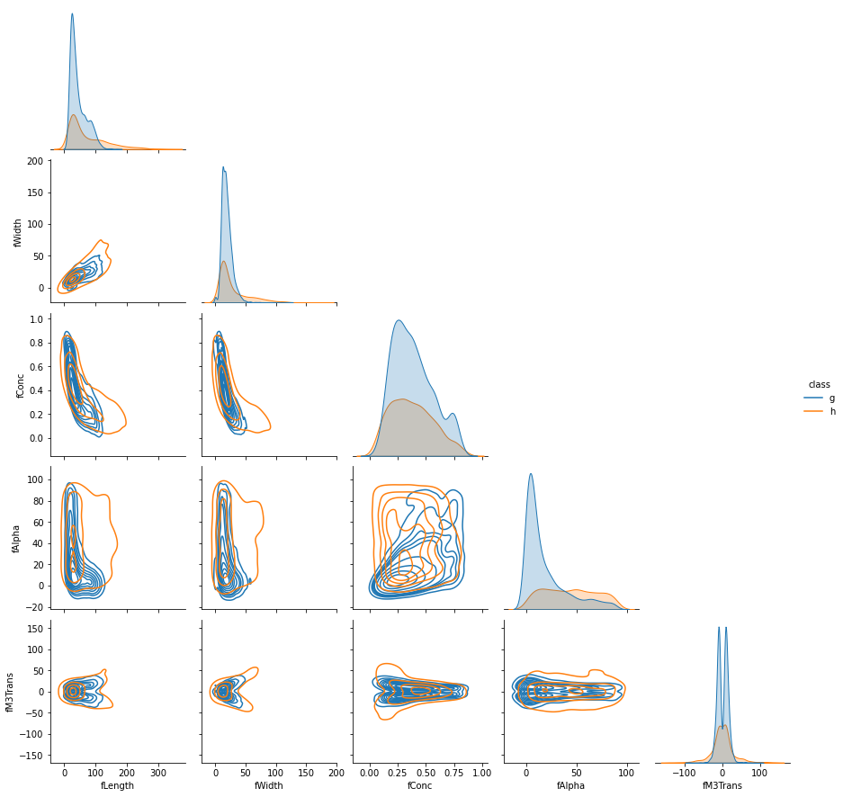
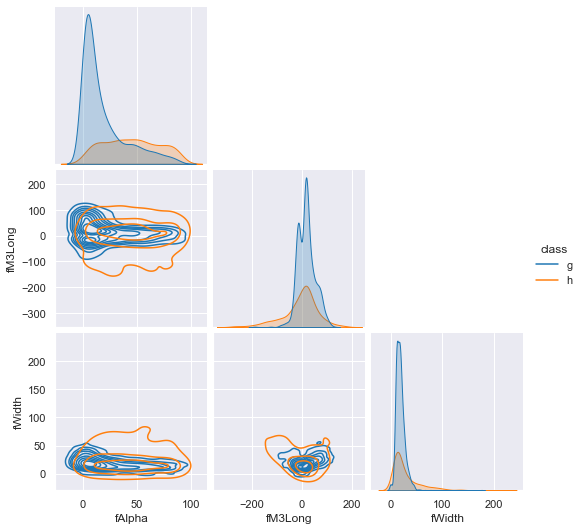
From this brief peek into the features broken down by target class ('g' for gamma, 'h' for hadron), one can see significant distribution overlap, which means that gamma detection will not be too easy, and there should be some uncertainty inherent in many predictions. Let's start by treating this as a typical binary classification problem.

Traditional ML Approach

What can a widely available, off-the-shelf solution do with this simple, but challenging dataset?

import numpy as np
from sklearn.ensemble import RandomForestClassifier
from sklearn.model_selection import cross_validate

X = df.drop(["class"], axis=1)
y = df["class"].replace({"g": 1, "h": 0})

rfc = RandomForestClassifier()
metrics = cross_validate(
    estimator=rfc,
    X=X,
    y=y,
    cv=5,
    scoring=["accuracy", "precision", "roc_auc", "average_precision"]
)
for m in metrics:
    print(f"{m}: {round(np.mean(metrics[m]), 3)} ± "
          f"{round(np.std(metrics[m]), 3)}")

Output:
fit_time: 3.48 ± 0.068
score_time: 0.114 ± 0.007
test_accuracy: 0.88 ± 0.004
test_precision: 0.885 ± 0.006
test_roc_auc: 0.935 ± 0.005
test_average_precision: 0.957 ± 0.004

Here we have instantiated and trained a tool (a Random Forest Classifier) for one specific task. Measured up against an evaluation set, it faithfully produces an excellent 88.5% precision — a good metric to focus on for a situation where you want to end up with a pure gamma sample to study.

But... what else can solutions like this accomplish? Let's give it a fair shake and cover feature importance, which can be extracted from a trained model. Without writing an entire tangent on caveats, cautions, and co-linearities, we can demonstrate the ability to derive impurity- and permutation-based feature importances.

import matplotlib.pyplot as plt
from sklearn.model_selection import train_test_split
from sklearn.inspection import permutation_importance

# Split the data and train a single model
X_train, X_test, y_train, y_test = train_test_split(
    X, y, test_size=0.33, random_state=314,
)
rfc = RandomForestClassifier()
rfc.fit(X_train, y_train)

# "Default" impurity-based feature importances
importances = rfc.feature_importances_
std = np.std([tree.feature_importances_ for tree in rfc.estimators_],
             axis=0)
indices = np.argsort(importances)[::-1]

# Permutation importance, which shuffles feature values to assess importance
pi = permutation_importance(
    estimator=rfc,
    X=X,
    y=y,
    scoring="average_precision"
)
pi_indices = np.argsort(pi["importances_mean"])[::-1]

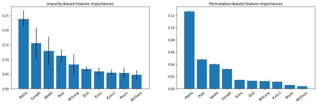
Here, we have trained an RFC and calculated some feature importances. The first is based on Mean Decrease in Impurity (MDI), using class impurity metrics internal to the decision trees. The second is permutation importance, which randomizes/shuffles the values in a single feature to see how much it affects performance. This type of inspection can lead to a better understanding of what drives the predictions made, and can better inform the user on certain details specific to the problem at hand.

There is also "partial dependence", which can be helpful in much the same way. The model can be exploited by artificially changing individual datum for single samples and measuring how that changes predictions.

from sklearn.inspection import plot_partial_dependence

plot_partial_dependence(
    rfc, X=X.sample(100), features=X.columns, n_cols=5,
)

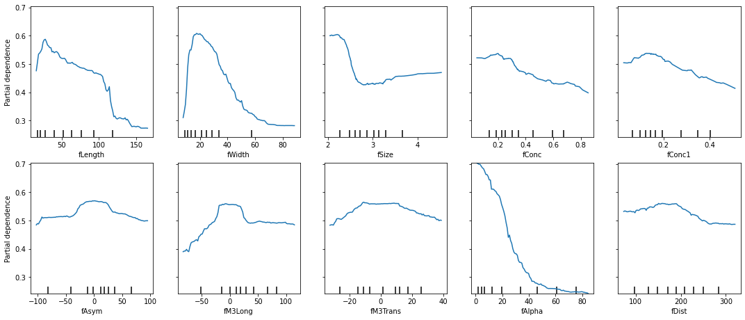
There are some great insights in plots like these that can tell you, "if this value is higher, then prediction probabilities of class 'g' drop," as is the case with fAlpha here.

And there we have it, a certainly not exhaustive, but fairly comprehensive assessment of what can do with a traditional ML model. One is required to specify the features and the target, train the model, and then one is able to:

1. Make predictions and evaluate them
2. Exploit the model to learn about how the features influence the prediction

... and that's about it. The problem is that this approach assumes:

• You will only care about the answer to this one question
• You don't care a whole lot about the input features
• You don't want any information pertaining to individual samples
• All of your data is anomaly-free, or you don't care about anomalous or surprising values influencing your predictions

There are certainly platforms out there that go the full Dr. Frankenstein and stitch together N different individual models to be able to describe each individual feature or do anomaly detection, but this can become inelegant, unwieldy, and generally unsatisfying.

Now that the lede has been sufficiently buried, let's take a look at what can be achieved if we take a step into a new world of holistically data-aware modeling as we find in Redpoll's Reformer Engine.

Redpoll's Reformer Engine

The Reformer engine runs as a server instance to which one can connect and make any number of requests. This has a number of benefits over maintaining, updating, and distributing a model file, but let's focus on task utility for the moment.

Let's begin with inference (prediction) of the target. With Reformer running on this set, inference, along with many other operations, is a simple matter to execute.

import reformer

# Create a client instance connected with the server
client = reformer.Client("0.0.0.0:8000", secure=False)

# Request imputed values for the test rows
y_pred_rp = client.impute(col="class", rows=X_test.index)
y_pred_rp.head()

Output:
       uncertainty class
18597     0.019604     h
16776     0.153241     g
15694     0.041106     g
16397     0.020332     h
3772      0.201858     g

Here's our first departure from what one might be used to seeing. Reformer, by default, pairs its individual inferences along with an uncertainty value. More on this later.

The evaluation of this set of predictions yields:

from sklearn.metrics import accuracy_score, precision_score
from sklearn.metrics import confusion_matrix

accuracy = accuracy_score(y_test, y_pred_rp)
precision = precision_score(y_test, y_pred_rp)

print(f"Test Accuracy: {round(accuracy, 3)}")
print(f"Test Precision: {round(precision, 3)}")
print(confusion_matrix(y_test, y_pred_rp))

Output:
Test Accuracy: 0.85
Test Precision: 0.86

         Predicted       Total
                 -     +
Actual -      1605   606  2211
       +       335  3731  4066
Total         1940  4337  6277

Feature importance can also be derived from the Reformer engine by calculating the proportion of information related to the target carried in each column.

ip_data = client.information_proportion(
    target_cols=["class"],
    predictor_cols=[col for col in df.columns if col != "class"]
)

fig = plt.figure(figsize=(12, 8))
sns.barplot(
    data=ip_data,
    x="Predictor",
    y="Information Proportion",
    color="#333333",
)

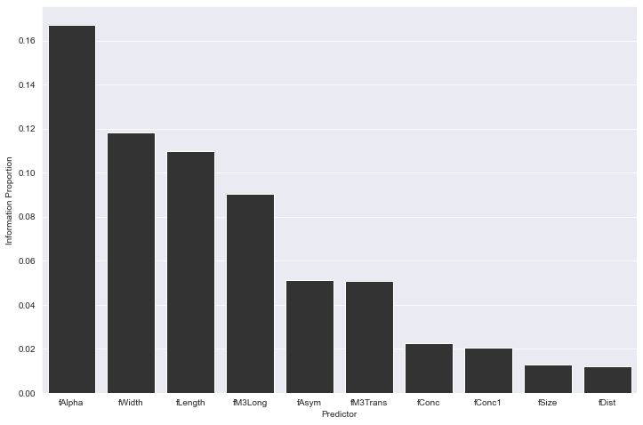
We see in this apples-to-apples evaluation that a stock RFC wins out, 88.5% to 86% on precision. If one is not participating in a Kaggle competition, eking out every point possible, and is able to tolerate this marginal difference, we can begin to explore the host of opportunities created with Redpoll's Reformer engine.

Beyond the Target

Let's turn our attention to how the Reformer engine has modeled the entire dataset. We consider a situation where a particularly energetic gamma ray has struck our hard disk and we have lost 1/3rd of all values in our dataset. To do so, we randomly select 33% of all data entries and set them to NaN.

import missingno as mno

missing_df = df.copy()

# Flatten all of the values into a single array
vals = missing_df.drop(["class"], axis=1).values.flatten()

# Select one third of them randomly
null_ixs = np.random.choice(
    range(len(vals)),
    size=round(len(vals)/3.0),
    replace=False
)
# Set these selected values to NaN
vals[null_ixs] = np.NaN

# Overwrite the values in the dataframe with this 1/3rd empty set
missing_df.iloc[:, :-1] = vals.reshape(missing_df.shape[0], missing_df.shape[1] - 1)
print(missing_df[["fLength", "fWidth", "fConc", "fAlpha"]].sample(5))

# Visualize the missing values in the dataset
# (Dark regions are present data, white is missing)
mno.matrix(missing_df)

Output:
       fLength  fWidth   fConc   fAlpha
id
11327  19.4348  7.3353  0.7744  60.2180
15902      NaN     NaN  0.3250      NaN
18111  52.5016  9.5828  0.3645  32.6580
9525   20.1855     NaN     NaN      NaN
18742  20.8995     NaN  0.7428  81.0387

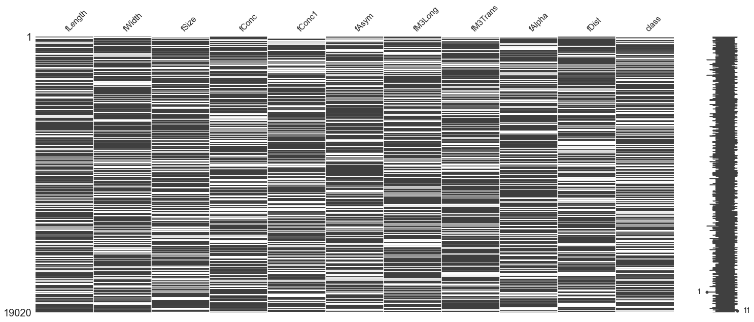
The result is this heavily redacted dataset. In the graphic above, imagine the entire dataframe compressed, with each horizontal line being a sample row. For each feature column, dark means that the data is present, and white means that this value is missing. Looking to the right, we see there's even a sample that has only one datum!

In this case of aggressive data loss, most traditional methods would have issues with managing to cope. Mean imputation or filling with sentinel values will keep things moving, or one might even go overboard and train individual models for predicting each feature.

Reformer, however, functions just as it did before without any issue. It is able to use whatever information is given in order to render a prediction. There is no behind-the-scenes value-filling going on; Reformer is simply able to make assessments based on what it does know.

y_pred = client.impute("class")

# Discard uncertainty value for now
y_pred = y_pred["class"]
y_pred = y_pred.replace({"g": 1, "h": 0})

print(f"Accuracy: {round(accuracy_score(y_test, y_pred), 3)}")
print(f"Precision: {round(precision_score(y_test, y_pred), 3)}")
print(confusion_matrix(y_test, y_pred))

Output:
Accuracy: 0.815
Precision: 0.813

         Predicted       Total
                 -     +
Actual -      1343   868  2211
       +       296  3770  4066
Total         1639  4638  6277

But, to go even further, imagine you did want to fill in the gaps as best you can. Go ahead and use the Reformer engine to make inferences on any feature in your dataset. Here, we impute all of the fLength values that have been removed and we evaluate the predictions by calculating the R2 score and plot the y_true - y_pred residuals.

from sklearn.metrics import r2_score

# Predict any missing values of *any* feature
y_pred_len = c.impute("fLength")["fLength"]

# Pull the true values from the full dataset
y_true_len = df.loc[y_pred_len.index, "fLength"]

# Calculate the evaluation metric of your choice
print(f"R2: {round(r2_score(y_true_len, y_pred_len), 3)}")

# Plot the residuals
fig, ax = plt.subplots(figsize=(12, 6))
sns.histplot(y_pred_len.values - y_true_len.values, ax=ax)
_ = ax.set_title("fLength Prediction Residuals")

Output:
R2: 0.81

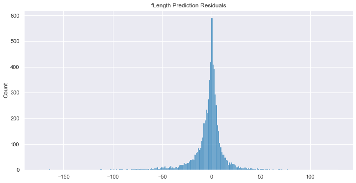
It bears repeating: Reformer has modeled the entire dataset. As such, it is able to make informed assessments with respect to each feature, not just the designated target. In fact, Reformer doesn't even ask you to designate a target when providing it data to work with.

Data-Aware

It's often the case that once our data is fed into fitting a model, we're done looking at it. Only the weights/parameters are saved. But what if your framework could help you be introspective about the data that you have.

Similarity

With Reformer, one can look to a single sample and find the most similar samples in the rest of the dataset. This is no basic euclidean or cosine distance calculation; those metrics are affected by scale. More importantly, what happens if an attribute's distribution is flat noise across the feature space? In that case, different values shouldn't matter so much with sample-to-sample similarity. Simple distances don't suffice when identifying similar samples.

Reformer, by contrast, cultivates an understanding of all of the features and samples in Model Space. This Model Space is robust, and (1) doesn't care about feature type (2) doesn't care if a feature is even present, and (3) understands the underlying conditional distributions, such as the flat noise feature example previously mentioned.

Here, we calculate the similarity between three arbitrarily chosen rows, and then we also scan through the dataset to find the most similar samples to row 0.

# Choose three arbitrarily rows
print(df.iloc[[0, 26, 15000]][["fLength", "fWidth", "fConc", "fAlpha", "class"]])

# Retrieve the similarity between pairs of rows
print(client.rowsim([["0", "26"], ["0", "15000"], ["26", "15000"]]))

Output:
       fLength   fWidth   fConc   fAlpha class
id
0      28.7967  16.0021  0.3918  40.0920     g
26     27.2304  19.2817  0.3710  77.5379     g
15000  37.9753   5.1561  0.6779  14.3465     h

    A      B  rowsim
0   0     26   0.625
1   0  15000   0.000
2  26  15000   0.000

# Find the most similar rows of all pairs in the dataset
all_pairs = [["0", str(i)] for i in range(1, len(df))]
top_matches = (client.rowsim(all_pairs)
     .sort_values("rowsim", ascending=False)
     .head())
print(top_matches)

Output:
       A      B  rowsim
4421   0   4422  1.0000
6516   0   6517  0.9375
11020  0  11021  0.9375
2396   0   2397  0.9375
657    0    658  0.8750

This functionality is not found in any traditional ML architectures. The closest that one might come to sample-sample similarity is if one were to compress the features to some kind of latent space and create a metric of distance in that learned space. This would generally not be a component of any standard classifier like the one used above, and would have to be built separately.

Anomaly Detection

Another data-aware strength with Reformer is the ability to understand when a value or sample is anomalous. Much like the similarity metric, this can be a complicated measure to define. Yes, if a value is several standard deviations outside of its distribution, it's anomalous — but it's also surprising if a gamma event has a high fAlpha angle value (see the jointplot at the top) even if the value isn't an outlier for the whole population.

Traditional solutions stand helpless to identify these for you before or even after training. There are plenty of standalone solutions and models that are designed specifically for anomaly detection, but then incorporating it significantly increases the complexity of the ML pipeline.

Reformer can natively highlight these samples for your consideration and evaluation. The statistical property of "surprisal" is used by Reformer to determine how surprising, unexpected, or anomalous a sample is. Here, we calculate the overall surprisal of each sample and fetch the most extreme one. We then plot the values of this anomaly over all of the base distributions.

from math import ceil, floor

# Calculate all the sample surprisals and fetch the most surprising
top_anomaly = (client.surprisal()
    .sort_values(by=["surprisal"], ascending=False)
    .iloc[0])

# Plot the values of this sample over the base distributions
fig, axs = plt.subplots(2, 5, figsize=(15, 5))
for i, col in enumerate(df.columns[:-1]):
    ax = axs[floor(i // 5)][i%5]
    sns.histplot(df[col], ax=ax, kde=True)
    ax.vlines(top_anomaly[col], 0, ax.get_ylim()[1], color='r')
fig.tight_layout()

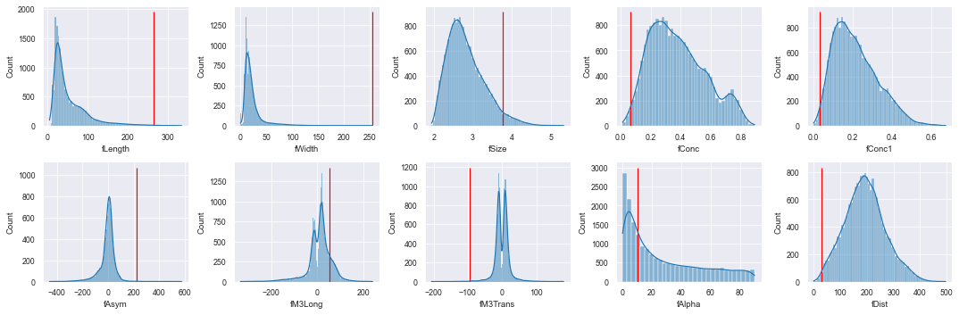
This anomaly, in most feature distributions, is plainly far into the tails. If acquainted with the domain at hand, this sample (and others up to a certain probabilistic level) can be evaluated to be either real or erroneous. Whether or not one might wish to keep an erroneous outlier in the training set is a judgment call, but one that can only be made once outliers have been identified.

This data-aware capability doesn't end there; it is possible to find samples that are anomalous with respect to a single feature or set of features. There can be cases where most of a sample's values are well within the realm of high probability, but feature X might be way off from what would be otherwise expected.

Here, we calculate the most surprising samples w.r.t. fWidth, and then fAlpha. We then plot these values over the base distribution.

# Calculate all the fWidth surprisals and get the top 5 most surprising
top_fwidth_anomalies = (client.surprisal("fWidth")
    .sort_values(by=["surprisal"], ascending=False)
    .head())
print(top_fwidth_anomalies)

Output:
         fWidth  surprisal
17717  256.3820  12.352112
17754  228.0385  10.388123
17619  220.5144   9.477771
17821  112.2661   8.524242
13496  201.3640   8.389742

This top anomaly is a trivial example of an outlier — its value is at the very fringe of the base distribution. It's the same sample as the one found above, and can be seen in the fWidth plot. This is not too interesting, but consider this next example:

# Calculate all the fAlpha surprisals and get the top 5 most surprising
top_falpha_anomalies = (client.surprisal("fAlpha")
    .sort_values(by=["surprisal"], ascending=False)
    .head())
print(top_falpha_anomalies)

ax = sns.histplot(df.fAlpha, kde=True)
_ = ax.vlines(12.4080, ymin=0, ymax=ax.get_ylim()[1])

Output:
        fAlpha  surprisal
12282  12.4080   8.358472
4462   89.9155   6.764617
11103  12.6281   6.717841
18038  89.7370   6.661253
12450  89.4816   6.628395

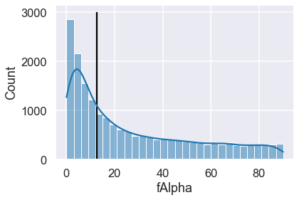
The top anomaly here is an interesting case where a particularly common fAlpha value of 12.4 is even more surprising than a sample with a fringe value of 89.9 — why is that? This is due to the context of the rest of the sample's data. We can get even more introspective about this anomaly by utilizing Reformer's simulation capabilities.

Simulation

While the MAGIC gamma ray dataset is itself a Monte Carlo (MC) generated sample, by training the Reformer engine with its data, Reformer itself can now act as a Monte Carlo generator. The MAGIC dataset is imbalanced, favoring gamma ray samples over hadronic 2-to-1. If, for whatever reason, a more balanced set is desired, downsampling of gamma events is a traditionally available option. Selecting the same hadron samples over again is also possible.

But what if we generate our own simulated hadron samples? With simulate(), it's possible to create new samples based on what we know about the features, and how they interact in Model Space. Specific values can be assigned as a "given" in this process.

Consider a case where we wish to simulate new hadronic samples; with the class value set to h. This is a simple one-line call.

# Generate new MC hadron samples
client.simulate(cols=df.columns[:-1], given={"class": "h"}, n=5)

Output:
     fLength     fWidth     fSize  ...    fM3Trans     fAlpha       fDist
0  94.632702  52.056796  3.673992  ...    9.237673  11.185377  137.102271
1  17.655791  10.795115  2.537168  ...   -5.829544  65.106615  134.789055
2  17.635636  73.751666  3.679984  ...  196.103052  52.722776  258.497931
3  45.758857   7.080488  2.647146  ...   -2.956160  65.282567  150.788139
4  43.598523  25.939003  2.922657  ...   13.998317  -0.488088  134.966457

Multiple givens can be assigned, allowing the user to simulate any hypothetical situation. Here, we simulate 500 new samples with two hypothetical givens.

simulation = client.simulate(
    cols=["fDist", "fConc", "class"],
    given={
        "fAlpha": 2.5,
        "fLength": 140,
    },
    n=500
)
simulation.head()

Output:
        fDist     fConc class
0  307.080782  0.243650     g
1  246.520126  0.329555     g
2  282.019657  0.188556     g
3  307.293975  0.231327     h
4  342.755502  0.225058     h

With this capability in hand, let's return to that anomalous fAlpha = 12.4 situation.

We fetch the attributes of that anomalous sample, and those are used to simulate 10,000 fAlpha values, given the rest of the sample values. Then we plot that distribution to gain insight into what the likely fAlpha distribution for one such sample is expected to be in Model Space.

# Get the non-fAlpha values from this sample
falpha_sample_data = df.loc[12282].drop("fAlpha").to_dict()

# Make 10k simulated values and plot the distribution
sim_alphas = client.simulate(
    cols=["fAlpha"],
    given=falpha_sample_data,
    n=10000,
)

# Plot the simulated fAlpha values
ax = sns.histplot(sim_alphas, kde=True)

# Plot the anomalous fAlpha value over the distribution
ax.vlines(12.4, ymin=0, ymax=ax.get_ylim()[1], color='r')

# Assuming gaussian-like distribution, plot std dev intervals
(mean, std) = (fa.mean(), fa.std())
ax.vlines(
    [mean-i*std for i in range(-3,4)],
    ymin=0,
    ymax=[ax.get_ylim()[1]*(0.4-(abs(i)*0.1)) for i in range(-3, 4)],
    color='gray',
)

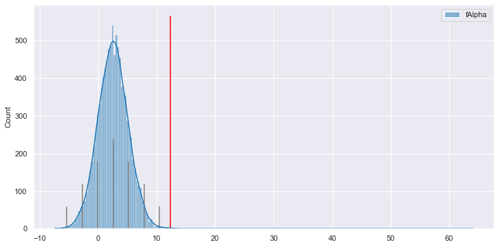
And here we have the awaited answer to "why is this perfectly average fAlpha value considered anomalous?" Given the rest of the data in the sample, according to Reformer's understanding of how all the features depend on and predict one another, fAlpha is expected to lie almost entirely between 0 and 10. A value of 12.4 is pretty surprising to Reformer, as you can see it's past the 3σ mark of the right tail.

Uncertainties

It's been touched on before, but let's talk about the ability to provide a measure of uncertainty. In a very similar procedure to the simulation method above, we ask for a prediction given limited information:

# Predict class, given two feature values
pred = client.predict(
    "class",
    given={"fConc": 0.17, "fDist": 110.0}
)
print(f"Prediction: {pred[0]}\nUncertainty: {round(pred[1], 3)}")

Output:
Prediction: g
Uncertainty: 0.195

The class g is predicted with an uncertainty value. This uncertainty metric is not a measure of feature-specific variance. It is instead a unitless metric specific to Redpoll's Reformer platform: 0.00 meaning no uncertainty, and 1.0 meaning maximum uncertainty. It is available as a way for it to communicate its confidence in an imputation or hypothetical prediction. This can be a very important metric to keep in mind when making critical decisions. Perhaps, depending on the circumstances, one might only want to take action when the certainty is high.

Let's give it some very clear hypotheticals and some confusing ones, too, to see what it returns. We use this jointplot as a reference.

• Here, values very likely to be a hadron shower are given. A low uncertainty prediction is expected.

pred = client.predict(
    "class",
    given={"fAlpha": 75.0, "fM3Long": -100.0, "fWidth": 75.0}
)
print(f"Prediction: {pred[0]}\nUncertainty: {round(pred[1], 3)}")

Output:
Prediction: h
Uncertainty: 0.015

• Values with high degree of overlap between gamma and hadron class are given next, which should report higher uncertainty without more information.

pred = client.predict(
    "class",
    given={"fM3Long": 0.0, "fWidth": 10.0},
)
print(f"Prediction: {pred[0]}\nUncertainty: {round(pred[1], 3)}")

Output:
Prediction:  g
Uncertainty: 0.223

• Next, we provide a likely gamma fAlpha value, but a likely hadronic fM3Long value. This contrast should increase the uncertainty of the prediction

pred = client.predict(
    "class",
    given={"fAlpha": 1.0, "fM3Long": -75.0},
)
print(f"Prediction: {pred[0]}\nUncertainty: {round(pred[1], 3)}")

Output:
Prediction: g
Uncertainty: 0.291

To provide a more intuitive understanding of what drives these predictions and uncertainties, let's assemble some visualizations. In Reformer's Model Space, there exist various views or perspectives on what distribution a datum might have. This is based on structure that Reformer has detected in the data. Various combinations of features may exhibit structure that Reformer can learn and use for inferences. Sometimes, the structures learned may be in agreement (or conflict) with each other for a particular sample.

In general, if all of these views in model space agree with each other for a given prediction, the uncertainty will be lower. If they wildly differ, a superposition of all of the distributions will provide a prediction, but the uncertainty will be elevated.

Now, choosing a random sample from our dataset (row 6), let's ask it what it would predict for a couple of its feature attributes. In these examples, we will see:

• Low uncertainty for the case of predicting fSize
• Medium uncertainty for predicting fAlpha
• High uncertainty for predicting fLength

client.render_uncertainty(
    col="fSize",
    row_ix="6",
)

client.render_uncertainty(
    col="fAlpha",
    row_ix="6",
)

client.render_uncertainty(
    col="fLength",
    row_ix="6",
)

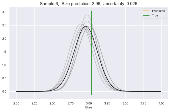
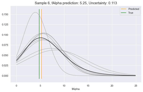
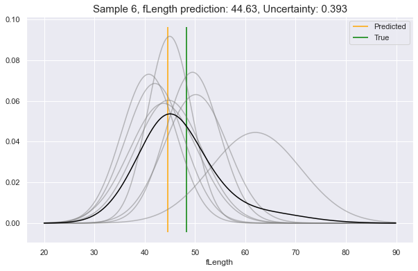
We see above, the gray lines constitute where the requested feature is likely to be, according to different perspectives in Model Space. The black line is the unification of all these underlying perspectives. The yellow vertical line is the predicted value, which will always be at the peak value of the black curve. This can be compared to the green vertical line: the true value.

As you see, the more that the Model Space perspectives agree on the predictive distributions, the lower the uncertainty, and vice-versa.

Conclusion

AI and machine learning is currently entrenched in a rather limited paradigm of functionality and scope. There exist entire toolboxes of "unit-taskers" that can successfully do one thing pretty well. I hope you have found in this post as evidence that a new paradigm is possible with the Reformer engine. One that can model an entire data set or domain and do many, many things well.

• Prediction (of all features)
• Work with missing data — and can intelligently impute absent values
• Provide feature importance
• Simulate new samples
• Detect anomalous whole samples
• Detect anomalous individual datum, given the context of the rest of a sample
• Provide uncertainty of predictions

This, in contrast to typical ML solutions which can only, on their own:

• Make predictions of one feature
• Provide feature importance of one feature
• Provide a kind of uncertainty/score as far as sigmoid or softmax values

And all of this is done not as some Frankenstein Suite of unrelated products and models, but as the result of exploiting all of the benefits that come from one platform understanding how it's all connected.

This is holistic, humanistic AI in action.